SARI

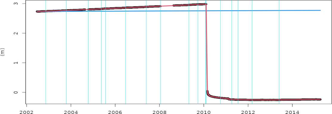
Estimated daily mean position changes at the CONZ00CHL (Chile) station in the east (positive) - west (negative) direction from the SPOTGINS solution.
On February 27, 2010, the Mw 8.8 Maule earthquake caused a co-seismic displacement of 293.2 ± 0.1 cm to the west at the station location. This was followed by a post-seismic displacement of 25.6 ± 0.1 cm over the subsequent years. The post-seimic deformation was interrupted by the Mw 6.9 Tomé earthquake on February 11, 2011, which added an additional 2.6 cm of displacement.
The red curve represents the fitted kinematic model, which consists of a linear trend, offsets, and exponential and logarithmic decays.
The blue line represents South America's mean plate motion extracted from the NNR-GSRM v2.1 model (Kreemer et al. 2014). The difference between the blue and red lines would represent the evolution of the observed local crustal deformation over time.
The vertical cyan lines represent equipment changes recorded in the station's sitelog. Antenna changes can sometimes introduce apparent instantaneous displacements due to calibration limitations, which may be similar in magnitude to small or moderate earthquakes.

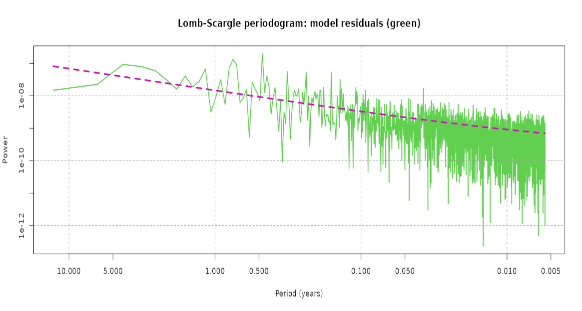
Green: power spectrum of the residual daily mean position time series obtained from the fitted model shown in the top figure.
The power spectrum shows the distribution of unmodelled series variability per unit of frequency along different periods of time. As is common with GNSS position series, the power of unmodelled long-period variations dominates the spectrum. The exact cause of this common spectral pattern is not fully understood, but the most likely suspect is related to orbit mismodelling.
The standard deviation of the residual series (not shown) is only 1.8 mm. This represents the precision or repeatability of the estimated daily mean positions with respect to the fitted kinematic model. That's about the width of a crayon point on a sheet of paper of tens of millions of km² constantly moving underneath (the plate).
Pink: power spectrum of the noise model fitted to the residual series using Maximum Likelihood Estimation (MLE).
The estimated noise model is composed of 0.9 ± 0.1 mm of white noise at short periods and 4.6 ± 0.2 mm of power-law noise with a spectral index (slope) of -1.04 ± 0.07. The estimated power-law noise corresponds to a flicker noise process that dominates the white noise; the resulting crossover period between both noise types is only 4 days and therefore, it is hardly visible on the power spectrum.
The estimated noise model allows obtaining a more accurate formal uncertainty of the linear trend by almost seventeen times, compared to an estimate assuming only white noise.

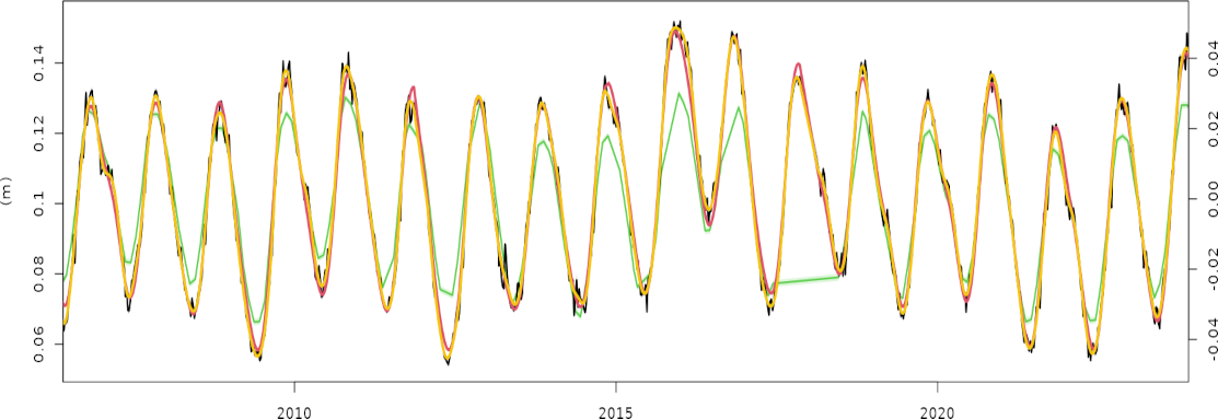
Black: weekly-averaged height change estimates at the NAUS00BRA (Brazil) station from the SPOTGINS solution.
Red: fitted Kalman filter model composed of a time-variable linear trend and a time-variable annual signal of amplitude between 1.8 and 4.1 cm.
Yellow: low-pass filtered weekly height changes using the Vondrak smoother.
Green: estimated monthly height changes at the same location from the GRACE NASA GSFC mascons solution obtained from the EOST loading service, for comparison purposes. The GRACE series are plotted on the right axis using the same scale as the GNSS series on the left axis.
While the GRACE estimated annual height changes at this site are in phase with the GNSS estimated annual height changes, their amplitudes do not match, being stronger for the GNSS height changes. Also the estimated interannual height variations are stronger for GNSS, with linear trend chages of ± 4 mm/year (not shown).
Both features may be explained, on the one hand, by the low spatial resolution of the GRACE estimates that does not allow accounting for the spatial distribution of water around the GNSS station in detail. On the other hand, while most of the annual variation of the GNSS height estimates could be explained by hydrology loading, the GNSS position estimaes integrate many proceses not related to hydrology loading. Therefore, a perfect match of the estimated height changes between GNSS and GRACE is not expected.

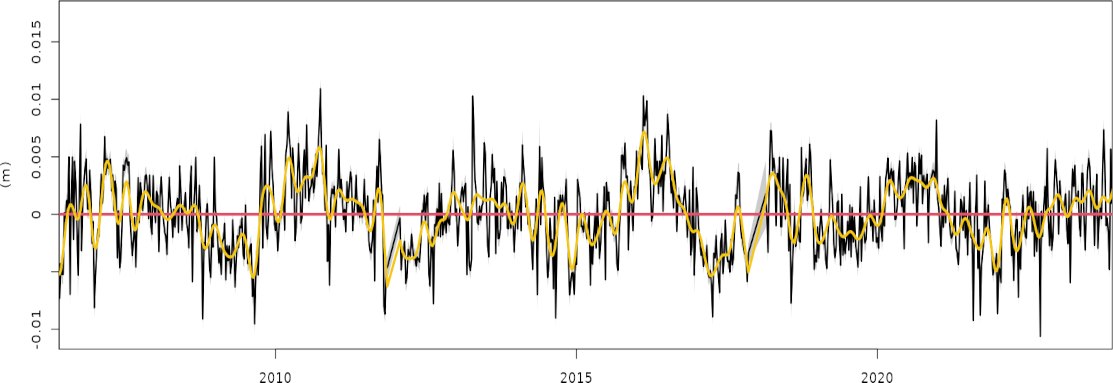
Black: weekly height differences between the GNSS position time series and the Kalman filter model shown in the top figure.
The standard deviation of the differences is 3.3 mm and most of it is concentrated at periods ranging from 2 to 5 years. The time-variable linear trend component of the Kalman filter model effectively captures most of the series variability for periods longer than about 5 years.
Yellow: weekly height differences between the Vondrak smoother and the Kalman filter model shown in the top figure. This is equivalent to computing the Vondrak smoother with the residual series of the Kalman filter model (black).

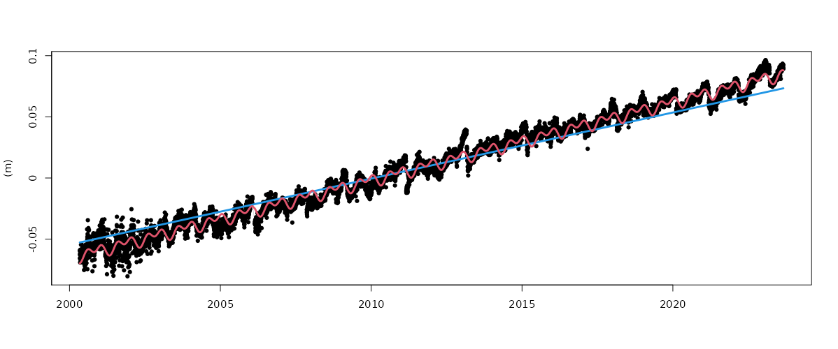
Black: daily height changes estimated at the YELL00CAN (Canada) GNSS station from the SPOTGINS solution.
Red: fitted model composed of a vertical uplift with an average value of 6.36 ± 0.17 mm/yr, and stationary annual and semi-annual variations of 3.1 and 3.3 mm, respectively.
The YELL00CAN station is installed on a concrete pillar anchored to exposed bedrock, which leaves the glacial isostatic adjustment (GIA) as the only possible ongoing process that could explain a constant uplift of this magnitude.
Blue: GIA uplift prediction extracted from the ICE-6G-ANU model (Purcell et al., 2016) at the station's location.
The GIA model accounts for 85 % of the estimated uplift, resulting in a significant linear trend difference of 1 mm/yr. The other two GIA models available in SARI show even greater differences: -1.2 mm/yr with the Caron and Ivins (2019) model, and +1.4 mm/yr with the ICE-6G-VM5a model (Peltier et al., 2018).
The spread of the available uplift predictions may be explained by the limitations of accurately modeling the near-field GIA process.

Black: daily height residuals between the corrected GNSS position time series and the fitted model of the top figure.
Before fitting model, the GNSS height series were corrected with a secondary series obtained from atmospheric, oceanic and hydrologic general circulation models available from the EOST Loading Service (EOSTLS server in SARI). Several models and their combinations were easily tested.
Non-tidal ocean loading corrections with the ECCO2 model barely reduce the estimated annual variation (4 %) or change the overall variability at other periods.
Soil moisture and snow loading corrections with the ERA5 reanalysis (ERAHYD product) produce a moderate reduction of the annual variation (19 %), but still do not affect the series variability at the rest of the observed periods significantly (1 % increase).
A much larger impact comes from the atmospheric loading corrections with the ERA5 reanalysis (ERA5IB product): 35 % reduction of the annual variation and 20 % reduction of the series variability at the other periods. Adding the dynamic response of the ocean to atmospheric pressure and winds (ERA5TUGO product) results in even better scores at this site: 37 % reduction of the annual variation and 26 % reduction of the series variability. Finally, the combination of atmospheric, oceanic and hydrologic loading corrections (ERA5TUGO & ERAHYD products) reduces the annual variation by 39 % and the series variability by 27 %.
However, the reduction of the series variability is not uniform, but concentrated in the frequency band extending from a few days to a few months. Reducing the variability at these periods facilitates the separation between uncorrelated white noise at short periods and time-correlated flicker noise at long periods, which otherwise would be evaluated as broadband power-law noise. Changes in the flicker noise content of a series are particularly relevant because this type of noise drives the assessment of the formal uncertainties of the estimated model parameters, especially the linear trend.
Overall, the predicted loading at this site reduces some of the estimated position variability at high frequencies, and that can help unveiling hidden features in the series, such as discontinuities or small periodic variations. However, it is clear that most of the series variability, including most of the prominent annual variation, is not explained by the current loading models. The residual variability may be related to the limitations of the loading models to account for all the spatial and temporal mass variations, specially for continental hydrology. In addition, the GNSS position estimates include other physical processes not related to mass loading, such as thermoelastic deformation of the groud and of the antenna mount. Finally, GNSS position estimates also include propagated processing errors that can originate from many sources: the reference frame, orbit dynamics, atmospheric refraction, and the radiation pattern of the ground antenna, to name a few.

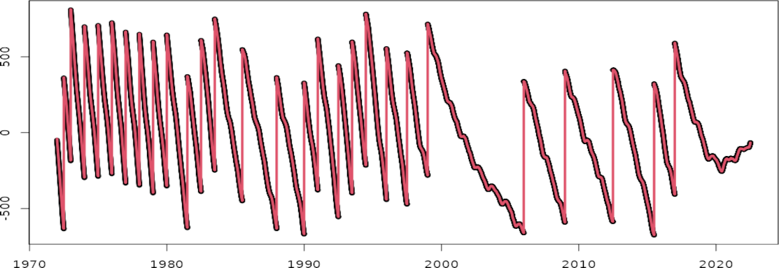
Black: daily UT1-UTC differences in milliseconds from the C0414 series of the IERS combined Earth orientation parameter solution.
Each discontinuity in the series represents a leap second added to the UTC time to maintain synchronization with the Earth's irregular rotation speed.
When the UT1-UTC differences remain stable around a constant value, it indicates that the Earth's rotation speed (given by UT1) matches the standard rotation speed of one revolution in 24 h (given by UTC). This is observed only around 2020 and during very short periods occurring with some regularity since 2000. The overall negative trend clearly shows that the Earth's rotation speed is generally slower than the standard speed, resulting in days slightly longer than 24 hours by a few milliseconds.
Red: Kalman filter model composed of a time-variable linear trend and leap second offsets on the dates indicated by the IERS Bulletin C. These leap second offsets were tightly constrained to their known value of 1000 milliseconds.
When the leap seconds are removed, the UT1-UTC series transforms into UT1-TAI series, which was then fitted with a time-variable linear trend. Changes in the UT1-TAI trend represent changes in the duration of the day (see the figure below).

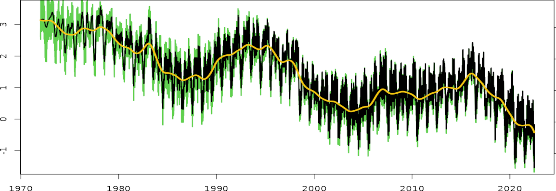
Black: the sign-reversed UT1-TAI time-variable linear trend estimate, from the Kalman fit of the top figure, transformed from ms/year to ms/day units.
The UT1-TAI rate with reversed sign is known as the excess of length of day (LOD). The zero value represents an Earth rotation of exactly 24 hours. A positive LOD value represents days longer than 24 hours in ms, and vice versa.
Green: the daily LOD series in ms/day from the official IERS C0414 combined solution, for comparison.
The seasonal trend variations in the UT1-TAI series were not properly accounted for by the a priori state variance and the process/observation noise ratio, so the Kalman filter takes some time to adjust.
Yellow: low-pass filtered daily LOD series using the Vondrak smoother.
While days have generally been longer than 24 hours over the observed period, a negative trend in the LOD series suggests that the Earth's rotation is accelerating, resulting in shorter days closer to the standard duration of 24 hours. In May 2020, the smoothed LOD series crossed into negative values, being the first time in the space geodesy era that the duration of the day is systematically shorter than 24 hours.

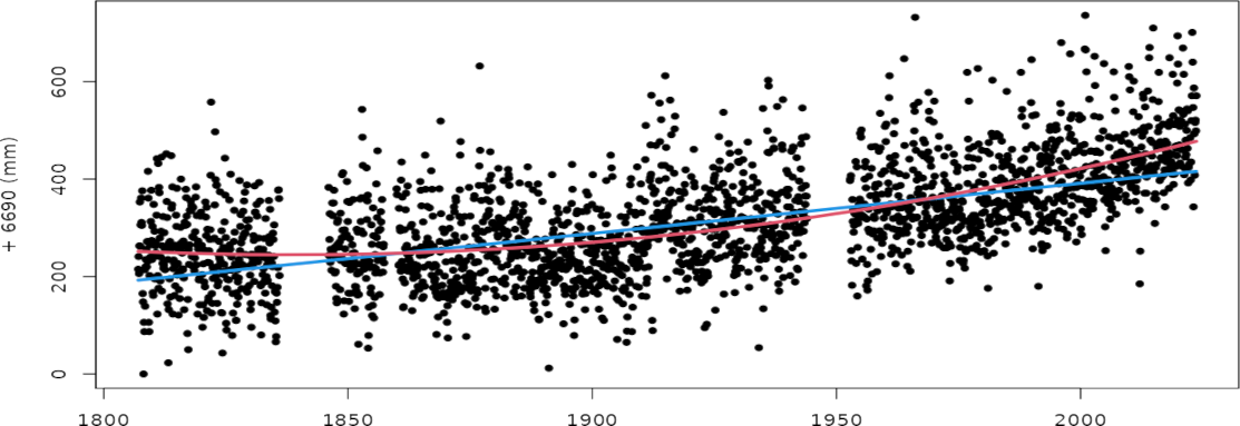
Black: monthly mean sea-level series at the Brest station since 1807 obtained from the PSMSL server. This is probably the world's longest geodetic record that is still in operation.
Blue: sign-reversed GIA vertical land motion extracted from the Caron and Ivins 2019 model: -1.03 mm/yr (subsidence).
The predicted GIA subsidence rate agrees well with multiple estimates of GNSS vertical land motion rates, with nearly 20 years of observations at this site, and with an average value of -0.78 ± 0.17 mm/yr (not shown).
Red: least-squares fit of a quadratic polynomial showing an average sea-level rise of 1.0 ± 0.1 mm/yr and an acceleration of 1.38 ± 0.04 mm/yr/century.
Due to this acceleration, the relative or coastal sea level is currently rising at approximately 2.5 mm/yr today, and could potentially exceed 5 mm/yr within the next 200 years if the estimated acceleration value remains unchanged.

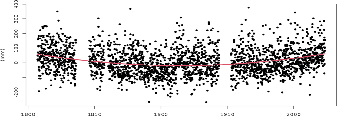
Same as the top figure, but the tide gauge record has been corrected for the inverse of the GIA subsidence rate before fitting the same least-squares model.
The estimated acceleration remains unchanged and, while the absolute or climate-driven mean sea-level rate is now close to zero, the banana shape of the series indicates a reversal in sea-level change at this site, from falling to rising, over the past two hundred years.
In addition, the histogram of the fit residuals (not shown) exhibits a slight skew towards higher sea levels, suggesting that extreme sea levels are abnormaly more likely, particularly towards the end of the series.